Drone Wars

The US is sending Ukraine 100 new Switchblade 300 loitering munition drones as a tiny part of the recent $800M military aid package. These are basically the early, practical predecessors of the slaughterbots Stuart Russell was so concerned about back in 2017.

The Switchblade 300 is about 2 feet long and weights about 2.5 kilograms, so perhaps 10x to 100x larger than a slaughterbot. Like the slaughterbot, the Switchblade uses a mass efficient shaped charge explosive, only much larger – suitable for destroying light military vehicles. And this is what makes the Switchblade actually practical: the primary purpose of modern warfare – at least as practiced by the West – is to disarm your opponent. Killing humans is oh so passe.

Current Switchblades are remote piloted, which along with the 10 km range, is a rather severe limitation and perhaps why we sent a relatively small package of only 100 units – this is probably a field test.

Full autonomy is an obvious next step. An iphone 13 class device weighs about 150 grams (and even less if the battery is reduced, as the UAV only has 10 minutes of flight time), and costs only about $1,000 vs $6,000 for the drone (the 600 model has a javelin anti-tank warhead and is 10x larger and costlier), so there are no significant tech or economic limiters on creating fully autonomous variants.

A fully autonomous Switchblade-like drone munition would not be tethered to a nearby operator through a short range radio link. Removing the tether limitation, the next limitation is the short 10 km range, which we could easily extend by utilizing cruise missiles as delivery platforms.

A cruise missile (either the trusty old Tomahawk or the newer stealthy JASSM) can deliver a 450 kg warhead up to 2,000 km, traveling a little below the speed of sound just 100 ft or so above the ground. A single cruise missile could thus deliver over 150 Switchblade 300 sized drones deep into enemy territory.

A single C-130 transport plane can carry up to 19 cruise missiles to the border of enemy territory, which can then launch in mid-air from crates ejected from the back of the plane – ie the “Rapid Dragon” program – to ultimately deliver almost 3,000 drones per transport plane. Each larger C-17 transport can carry 75 cruise missiles, or over 10,000 of the smaller SB-300 drones or 1,000 of the larger SB-600 drones. For point of comparison, a single volley of 10,000 drones could probably destroy or disable most of the Russian military’s transport/logistics trucks, and a volley of 1,000 of the larger drones could destroy a good chunk of their main battle tanks.

A dozen of these massive Globemasters could carry over 100,000 drones, enough to end most armies in a single volley.

If each drone costs $6,000, the cruise missile delivery adds another $9,000 in unit cost, and transport plane delivery then adds another $8,000 up front and less than $1,000 for amortized fuel, for a total cost rounding up to ~$15,000 per delivered munition and end inflicted light vehicle casualty, or perhaps ~$150,000 for every battle tank casualty (all assuming a high lethality ratio, which seems to be the case today against forces that do not have counters for these small fast drones, and nobody yet has counters for large masses of drones).

This is potentially a paradigm shatterer – a 100x efficiency improvement in destroying light vehicles. Cruise missiles, priced a bit over $1M a pop, are simply too expensive to use against such numerous small targets.

A future Rapid Dragon using SpaceX Starship could deliver a bit more than a C-17 to any location in the world in less than an hour: deploying a suitable reentry vehicle near some undefended border air space which launches 100 cruise missiles that then deliver up to 15,000 drones a further 2,000 km into enemy territory.

Warfare is all about delivering minimal sufficient destructive energies to specific weakpoints in specific machines which are critical for the enemy’s war effort. Nuclear weapons are extraordinarily powerful, but just as extraordinary wasteful and inefficient. A vastly smaller minuscule amount of net destructive energy, but delivered with ultra high precision and focused on exactly the right locations, can do vastly more useful damage. The key enabler: Moore’s Law.

Brain Efficiency: Much More than You Wanted to Know

link post

TLDR: Brains are operating near a Pareto optimal frontier, mainly dominated by energy efficiency constraints; meanwhile Moore’s Law is quickly nearing its own asymptotic endgame as it approaches the same physical constraints.

Magna Alta Doctrina

My latest lengthy post on Deep Learning is here on less wrong. Cross posting here once I get the Latex math working in wordpress.

AGI is Near(er)

A ‘common’ simple fermi estimate for the net computation required to produce AGI is something like:

HB * HL * X

Where HB is the compute equivalent of a human brain in ops/s, HL is the human lifetime, and X is some nebulous multiplier representing the number of experimental trials required to discover the correct architecture. Let’s call this the HumanBrain*HumanLifetime*X model.

HL – the human lifetime, shouldn’t be too controversial: it’s about 10^9 seconds for 32 years.

Joseph Carlsmith from Open Philanthropy has penned an impressively encyclopedic article seeking solely to estimate HB, resulting in a (sort of distribution with a ) median estimate of 10^15 op/s. That’s not far from the simple estimate of average synaptic spike rate * number of cortical synapses (ie ~1hz * 10^14 synapses =~ 10^14 op/s). My own estimate is similar, but with less variance (higher confidence).

A current high end GPU, the RTX 3090, has about 3×10^9 transistors that cycle around 1.5 x 10^9 hz for a maximum total circuit binary op throughput of ~5×10^18 ops/s. Is this surprising? However in terms of actual useful logic ops the max throughput (for 1 bit matrix multiplication using tensorcores) is closer to 10^15 op/s, or 10^14 flop/s for half floating point.

Although it may seem surprising at first to suggest that a current consumer GPU has raw compute power equivalent to the human brain, keep in mind that:

1. Synaptic ops are analog operations and thus intrinsically more equivalent to and expensive as lower bit flops – ie equivalent to 10^3 to 10^4 simple bit ops
2. The brain only uses 10 watts vs 350 for the GPU
3. Energy cost depends on wiring transit length which is longer in the brain
4. Consequent on 3.), the GPU max performance listed here only applies when using registers or smem, corresponding to minimal (and less useful) wiring length
5. Moore’s law is approaching end game for most relevant dimensions ( including the crucial bitop/J )
6. It’s fairly obvious that the brain pushes physical limits (biological cells are actual practical nanobots operating near the Landauer Limit¹)
7. The convergence of 5 and 6 in the near-term implies AGI

The GPU has about 3 OOM less total memory capacity, but GPUs can be networked together at vastly higher bandwidths, allowing one to spread a large model (virtual brain) across many GPUs (model parallelism) while also running many ‘individual’ AI instances simultaneously on each GPU (data parallelism). A fully analysis of how various net bandwidths compare (including compression) and will differentially shape AGI vs brain development is material for another day, but for now, just trust me that memory and interconnect aren’t hard blockers.

The HB*HL component forms a useful 2D product space. For the same given amount of compute, you can scale up your model complexity by a factor of X at the cost of reducing training data/time by X or vice versa.

AlphaZero models are much small than the brain, but are trained much faster than real-time, reaching superhuman capability in Go or Chess after <24 hours of wall-clock training time on a few thousand TPUs (~GPUs for our purposes), or < 100,000 GPU-hour equivalent, which is fairly close to HB*HL. (Note that AlphaZero did not use human knowledge, which makes the comparison more impressive)

GPT-3 is also smaller than the brain, and was trained for much longer in virtual time/data, but in terms of total compute was trained using just a few hundred GPU-years (ie, within one OOM of HB*HL). No, GPT-3 is clearly not a proto-AGI, as it wasn’t trained to be that. It was instead trained on the naively narrow task of sequential token prediction (and without the obvious human-like advantage of symbolic grounding through a sensori-motor world model – which yes obviously Google and OpenAI are now working as it’s obvious).

EfficientZero achieves superhuman test performance on the Atari 100k Benchmark, after only about 2 hours of virtual playtime (and thus superhuman sample efficiency!), which is especially impressive given that it doesn’t use visual pretraining (whereas humans have years of pretraining before ever trying Atari). It does this by learning an approximate predictive world model (of Atari) – ie using model-based RL. (the devil of course is in the details, but it’s much less obvious that EfficientZero isn’t simple proto-AGI). However it runs at about 0.3x real-time, so that 2 hours of virtual training takes roughly 6 hours of real time on 4 GPUs – so again within an OOM of the human training compute (ignoring human pretraining) .

The general lesson here is that DL systems are approaching human capabilities on interesting tasks when trained using roughly comparable amounts of total compute (with much more flexibility in the 2D space of model size vs training time tradeoffs).

So with those examples fresh in mind, what is a good guess for X – remaining experiments until AGI-GO-BOOM?

One simple prior (I internally name the Doomsday prior, but aka as the Lindy Prior), is to assume the # remaining experiments is similar to the # of similar-experiments conducted to date. We could roughly estimate #experiments by equating experiments to DL papers!

Eyeballing the graph above suggests an X estimate < 100k or less. (For point of comparison, naively applying the doomsday prior directly to years of research (assuming DL is a path ending with AGI) suggests AGI in a decade or two). If we instead use total number of papers (in any field) ever uploaded to arxiv as our prior for X, that only gets us up to about 1M.

Plugging 100k for X into HB*HL*X gives an estimate of ‘only’ about 28 billion GPU hours, or about $28 billion using (currently high) prices of $1/hr for an RTX 3090 on Vast.ai (recall 1 brain ~ 1 GPU ). For point of comparison, this is similar to the total amount spent on useless ethereum hashes in just one year. And naturally the larger estimate of $280 billion still isn’t so humongous in the grand schemes of nation-states and trillion dollar megacorps. These costs estimates are also conservative in assuming no further improvements from Moore’s Law.

At the end of the day though, what will matter most is net efficiency of spend. There is enormous room for further software improvements, such that these estimates are probably wildly over conservative. Besides further obvious significant improvements to low level matrix operations on GPUs (leveraging sparsity), we can vastly accelerate progress through advancements in meta-learning, and by doing most of the architecture search over small fast models/worlds. That latter sentence is mostly just a re-statement of the current reality, but the intertwined research tracks of sparsity and meta-learning will truly revolutionize research this decade – sharply curving all trendlines. Much more on that later.

¹ As a first hint, the energy currency of biology is ATP, and 1 ATP ~ 0.3 eV, within an OOM of room temp Landauer Limit of ~0.03 eV. Cells only use a few ATP to copy each base pair during DNA replication. As one electron volt is an electron with potential energy of 1 volt, the 0.03 eV Landauer Limit is a thermal noise barrier of 30 mV for electric computational systems like neural circuits. The typical neuron membrane resting potential is -70 mv, or only about 2X the limit, and it only cycles by another factor of 2x or so during action potentials. Digital computers operate at 10x or higher voltages, for higher speed and reliability.

COVID-19 in Iceland

12/06/2021 Update: This simple Iceland covid predictive model from early 2020 held up surprisingly well. My mean predicted Iceland IFR was 0.17%. As of today the actual total IFR is 0.179% (36 deaths / 20,044 confirmed infections). My predictions for the US were not as successful (off by a factor of ~3), mostly because I overweighted this Iceland based model. Iceland is a more homogeneous (and high vitamin-D) population than the US.

A private company in Iceland, deCODE genetics, has provided valuable insight into true COVID-19 prevalence by PCR testing a random-ish sampling of Icelanders.  You can clearly see the difference in the data itself: deCODE’s tests have a positive rate of ~0.9% which is about 10x lower than the positive rate of NUHI (a state hospital), as the latter is using a more standard biased testing strategy. This suggests that at least 0.9% of the Icelandic population has been infected with COVID-19. (The PCR test can’t reveal individuals who now have low viral levels.)

That’s at least 3.2K infections (0.9% of their population of 440K), and more realistically 4K to 5K.

Iceland has only 2 deaths so far for a naive IFR in the range of 0.04% to 0.2% to (we can probably ignore false negatives for deaths – as they are harder to miss in Iceland). Iceland’s cumulative case count is clearly in a linear growth regime (past midpoint of sigmoid). They have 6 patients in ICU (Iceland data), which has about a 30% fatality rate, and 19 in hospital with a 10% fatality rate so we can estimate the future total death count from this cohort in the 2 to 8 range.

This results in a mean predicted IFR of 0.17% (6/3500)and a range of 0.04% to 0.4% (2/5k to 8/2k), similar to influenza but potentially a bit (2x) higher. The uncertainty range will eventually tighten as we know more about survival in their current hospitalizations.

This agrees with the Diamond Princess data which rules out IFR much higher than influenza. (see my analysis here, or a more detailed analysis here) In that same post I also arrived at a similar conclusion by directly estimating under-reporting (the infection/case ratio) by comparing the age structure of confirmed cases to the age structure of the population and assuming uniform or slightly age-dependent attack rates similar to other viruses. That model predicts under-reporting of ~20X or more in the US, so it’s not surprising that the under-reporting in Iceland is still in the ~4X range.

Roughly let’s conservatively guess that a large fraction of the recovered were hospitalized previously, for 40 total hospitalizations. That’s a hospitalization rate of 1% (40 / 4,000), which is a little less but close to the CDC estimated influenza hospitalization rate of ~ 1.7% (500K hospitalizations / 29M infected for 2016).

This also puts bounds on how widespread C19 can be – with IHR and IFR both similar to influenza, there couldn’t be tens of millions of infected in the US as of a few weeks ago or we would be seeing considerably more hospitalizations and deaths than we do.

Covid-19 vs Influenza

EDIT: 11/18/2021 – With a death total rounding up to 1M, the true IFR in the US is probably around or over 0.5%, beyond my worst case estimates here.  My model was a better predictive fit for places like Iceland – and I oversampled from such places and failed to predict the high mortality rates in certain demographics.  (The striking geographic & demographic population differences in mortality probably stem more to differences in vitamin D and genetics rather than public policy.)

Covid-19 is either the greatest viral pandemic since the Spanish Flu of 1918 or it’s the greatest viral memetic hysteria since .. forever?  The Coronavirus media/news domination is completely unprecedented – but is it justified?

For most people this question is obvious – as surely the vast scale of ceaseless media coverage, conversation, city lockdowns, market crashes, and upcoming bailouts is in and of itself strong evidence for the once-in-a-generation level threat of this new virus; not unlike how the vast billions of daily prayers to Allah ringing around the world is surely evidence of his ineffable existence. But no – from Allah to evolution, the quantity of believers is not evidence for the belief.

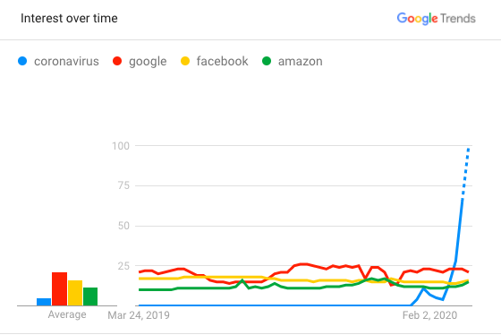
“Coronavirus” has recently become the #1 google search term, beating even “facebook”, “amazon”, and “google” itself.  Meanwhile a google search of “coronavirus vs the flu” results in this knowledge-graph excerpt:

Globally, about 3.4% of reported COVID-19 cases have died. By comparison, seasonal flu generally kills far fewer than 1% of those infected.

Which is from this transcript of a press briefing by the WHO Director-General (Tedros Adhanom Ghebreyesus) on 3/3/2020. This sentence is strange in that Ghebreyesus was careful to use the word ‘reported COVID-19 cases’, but then compared that COVID-19 case fatality rate (CFR) to the estimated infection fatality rate (IFR) for flu of ‘far fewer than 1%’. What he doesn’t tell you is that the CFR of seasonal influenza is actually over 1%, but the estimated true IFR is about two orders of magnitude lower (as only a small fraction of infections are tested and reported as confirmed cases). If there was a live tally of the current Influenza season in the US, it would currently list ~23,000 deaths and 272,593 cases, for a CFR of ~8%.

The second google result links to a reasonable comparison article on medicalnewstoday.com which cites a situation report from the WHO, which states:

Mortality for COVID-19 appears higher than for influenza, especially seasonal influenza. While the true mortality of COVID-19 will take some time to fully understand, the data we have so far indicate that the crude mortality ratio (the number of reported deaths divided by the reported cases) is between 3-4%, the infection mortality rate (the number of reported deaths divided by the number of infections) will be lower. For seasonal influenza, mortality is usually well below 0.1%. However, mortality is to a large extent determined by access to and quality of health care.

This statement is mostly more accurate and careful – it more clearly differentiates crude case mortality from infection mortality, and notes that the true infection mortality will be lower (however, according to CDC estimates seasonal flu IFR is not ‘well below’ 0.1%, rather it averages ~0.1%). So where is everyone getting the idea that covid-19 is much more lethal than the flu?

Apparently – according to it’s own author – a blog post called “Coronavirus: Why You Must Act Now” has gone viral, receiving over 40 million views. It’s a long form post with tons of pretty graphs.  Unfortunately it’s also quite fast and loose with the facts:

The World Health Organization (WHO) quotes 3.4% as the fatality rate (% people who contract the coronavirus and then die). This number is out of context so let me explain it. . .. The two ways you can calculate the fatality rate is Deaths/Total Cases and Death/Closed Cases.

No, the WHO did not quote 3.4% as the true fatality rate, and no that is not how any competent epidemiologist would estimate the true fatality rate, and importantly – that is not how the off-cited and compared 0.1% influenza fatality rate was estimated.

How Not to Sample

There is an old moral about sampling that is especially relevant here: if you are trying to estimate the number of various fish species in a lake, pay careful attention to your lines and nets.

For the following discussion, let’s categorize viral respiratory illness into 5 categories:

• 0: uninfected
• 1: infected, but asymptomatic or very mild symptoms
• 2: moderate symptoms – may contact doctor
• 3: serious symptoms, hospitalization
• 4: severe/critical, ICU
• 5: death

If covid-19 tests are only performed post-mortem (sampling only at 5), then the #confirmed_cases = #confirmed_deaths, and case fatality rate (CFR) is 100%.  If covid19 tests are only on ICU patients, then CFR ~ N(5)/N(4+) , the death rate in ICU.  If covid19 tests are only on hospital admissions, then CFR ~ N(5)/N(3+), and so on.  The ideal scenario of course is to test everyone – only then will confirmed case mortality equal true infective mortality, N(5)/N(1+).

The symptoms of covid-19 are nearly indistinguishable to those of ILI (Influenza-like-Illness), which acknowledges that many diverse viral or non-viral conditions can cause a similar flu-like pattern of symptoms. Thus covid-19 confirmation relies on a PCR test.

When testing capacity is limited, it makes some sense to allocate those limited testkits to more severe patients.  Testing has been limited in the US and Italy – which suggests very little testing of patients at illness levels 1 and 2.  In countries where testing is more widespread, such as Germany, Iceland, Norway and a few others, the crude case mortality is roughly an order of magnitude lower, but even in those countries they are probably testing only a fraction of patients at level 2 and a tiny fraction of those at level 1 (who by and large are not motivated to seek medical care).

That Other Pandemic

In 2009 there was an influzena pandemic caused by a novel H1N1 influenza virus (a descendant variant of the virus that caused the 1918 flu pandemic). According to CDC statistics, by the end of the pandemic there were 43,677 confirmed cases and 302 deaths in the US ( a crude CFR of 0.7%) – compare to current (3/24/2020) US stats of 50,860 covid-19 confirmed cases and 653 deaths.  From the abstract:

Through July 2009, a total of 43,677 laboratory-confirmed cases of influenza A pandemic (H1N1) 2009 were reported in the United States, which is likely a substantial underestimate of the true number. Correcting for under-ascertainment using a multiplier model, we estimate that 1.8 million–5.7 million cases occurred, including 9,000–21,000 hospitalizations.

Later in the report they also correct for death under-ascertainment to give a median estimate of 800 deaths. So their median predicted IFR is ~0.02%, which is 35 times lower than the CFR (and 5 times lower than the estimated mortality of typical seasonal flu).

What’s perhaps more interesting is how (retrospectively) terrible early published mortality estimates were in hindsight: (emphasis mine)

We included 77 estimates of the case fatality risk from 50 published studies, about one-third of which were published within the first 9 months of the pandemic. We identified very substantial heterogeneity in published estimates, ranging from less than 1 to more than 10,000 deaths per 100,000 cases or infections. The choice of case definition in the denominator accounted for substantial heterogeneity, with the higher estimates based on laboratory-confirmed cases (point estimates= 0–13,500 per 100,000 cases) compared with symptomatic cases (point estimates= 0–1,200 per 100,000 cases) or infections (point estimates=1–10 per 100,000 infections).

So what about that 0.1% flu mortality statistic?

The off-quoted 0.1% flu mortality probably comes from the CDC, using a predictive model described abstractly here.  In particular, they estimate N(1+), the total number of influenza infections, from the number of hospitalizations N(3+) and a sampling driven estimate of the true hospitalization ratio N(1+)/N(3+):

The numbers of influenza illnesses were estimated from hospitalizations based on how many illnesses there are for every hospitalization, which was measured previously (5).

Some people with influenza will seek medical care, while others will not. CDC estimates the number of people who sought medical care for influenza using data from the 2010 Behavioral Risk Factor Surveillance Survey, which asked people whether they did or did not seek medical care for an influenza-like illness in the prior influenza season (6).

Hopefully they will eventually apply the same models to covid-19 so we can at least have apples-to-apples comparisons, although it looks like their influenza model estimates also leave much to be desired. In the meantime there are a number of other interesting datasets we can look at.

A Tale of Two Theories:

Let’s compare two plausible theories for covid19 mortality:

• Mainstream: Covid19 is about 10x worse/lethal than seasonal influenza
• Contrarian: Covid19 is surprisingly similar to seasonal influenza

First, let us more carefully define what “10x worse/lethal” means, roughly.  Recall that the true infective mortality is the unknown difficult to measure ratio N(5)/N(1+) – the number of deaths due to infection over the actual number infected. That ratio is useful for doing evil things such as estimating the future death toll of a pandemic by multiplying by the attack rate N(1+)/N – the estimated fraction infected.

We can factor out the death rate as the product of the fraction progressing to more severe disease at each step:

N(2+)/N(1+) * N(3+)/N(2+) * N(4+)/N(3+) * N(5)/N(4+)

So there are numerous means by which covid19 could have a 10x higher overall mortality than influenza.  For example it could be that only N(5)/N(4+) is 10x higher (the fatality rate given ICU admission), if for example covid19 is much harder to treat in ICU.  Or it could be that all the difference is concentrated in N(2+)/N(1+): that covid19 has a very low ratio of mild or asymptomatic patients. A priori, based on cross comparisons of other respiratory viruses (ie cold vs flu), it seems more likely that the any difference between covid19 and influenza is probably spread out across severity (the lower mortality of the common cold vs flu is spread out across a lower rate of serious vs mild illness, lower rate of hospitalization, lower rate of ICU, lower rate of death, etc).

Here is a collection of estimates for various hospitalization, ICU, and death ratios for influenza and covid19 ( N(C) denotes the number of lab confirmed cases ) :

• Influenza N(5)/N(3) ~ 0.07 (CDC 2018-2019 US flu season estimates)
• COVID-19 N(5)/N(3) ~ 0.08-0.10 (CDC COVID-19 weekly report table 1)
• Influenza N(4)/N(3) ~ 0.23 (Beumer et al Netherlands hospital study)
• COVID-19 N(4)/N(3) ~ 0.23-0.36 (CDC)
• Influenza N(5)/N(4) ~ 0.38 (Beumer et al)
• COVID-19 N(5)/N(4) ~ 0.29-0.36 (CDC)
• 2009 H1N1 N(3)/N(C) ~ 0.11 (Reed et al CDC dispatch)
• 2019 Flu     N(3)/N(C) ~ 0.07 (CDC Influenza Surveillance Report)
• COVID-19   N(3)/N(C) ~ 0.20 (CDC)

Note that the influenza data for hospitalization outcomes comes from two very different sources (CDC estimates based on US surveillance vs data from a single large hospital in the Netherlands), but they agree fairly closely: about a quarter of influenza hospitalizations go to ICU, a bit over a third of ICU patients die, and thus about one in 12 influenza hospitalizations lead to deaths.  The COVID-19 ratios have somewhat larger error bounds at this point but are basically indistinguishable.

The N(3)/N(C) ratio (fraction of confirmed cases that are hospitalized) appears to be roughly ~2x higher for covid-19 compared to influenza, which could be caused by:

• Greater actual disease severity of covid-19
• Greater perceived disease severity of covid-19
• Selection bias differences due to increased testing for influenza (over 1 million influenza tests in the US this season vs about 100k covid-19 tests)

So to recap, covid-19 is similar to influenza in terms of:

• The fraction of hospitalizations that go to ICU
• The mortality in ICU
• The overall mortality given hospitalization
• The overall mortality of confirmed cases

The mainstream theory (10X higher mortality than flu) is only compatible with this evidence if influenza and covid-19 differ substantially in terms of the ratio N(1+)/N(C) – that is the ratio of true total infections to laboratory confirmed cases, which seems especially unlikely in the US given it’s botched testing rollout with covid-19 testing well behind influenza testing. If covid-19 is overall more severe on average, that could plausibly lead to a lower N(1+)/N(C) ratio, but it seems unlikely that the increase in severity is all conveniently concentrated in the one variable that is difficult to measure.

The Diamond Princess

Sometime in late January covid-19 began to silently spread through the mostly elderly population onboard the Diamond Princess cruising off the coast of Japan. The outbreak was not detected until a week or two later; a partial internal quarantine was unsuccessful.  The data from this geriatric cruise ship provides a useful insight into covid-19 infection in an elderly population as most all 3,711 passengers and crew were eventually tested.

Now that it has been almost two months since the outbreak the outcome of most of these cases is known. However, worldometers is still reporting 15 patients in serious/critical state. I’ve pieced together the age of deaths from here and news reports, but there are 2 recent deaths reported from Japan of unknown age. Thus I’ve given an uncertainty range for the 2 actual deaths of unknown age and an estimate of potential future deaths based on the previously discussed ~30% death ratio for ICU patients. I pieced together flu age mortality from 2013-2014 flu season CDC data here and from livestats and provided 95% CI binomial predictions. The 2013 flu season was typical overall but somewhat higher (estimated) mortality in the elderly. The final column has predictions using covid-19 CDC case mortality.

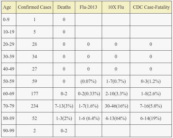
The observed actual death rates are rather obviously incompatible with the theory that covid-19 is 10x more lethal than influenza across all age brackets in this cohort.

The observed deaths is close to the Influenza-2013 predictions except for the 7 (or a few more) deaths in the 70-79 age group which is about ~2x higher than predicted. The CDC case mortality model predictions are much better than 10x flu, but are still a poor fit for the observed mortality.  More concretely, the Influenza-2013 model has about a 100x higher bayesian posterior probability than the CDC case fatality model. The latter severely overpredicts mortality in all but the 70-79 age bracket.

One issue with the Diamond Princess data is that a cruise ship population has it’s own sampling selection bias. Of course this is obviously true here in terms of age, but there also could be bias in terms of overall health. People in the ICU probably aren’t going on cruises. On the other hand, cruises are not exactly the vacation of choice for fitness aficionados.  It seems likely that this sampling bias mostly affects the tail of the age distribution (as the fraction of the population with severe chronic illness preventing a cruise increases sharply with age around life expectancy) and could explain the flatter observed age mortality curve and low deaths in the 80-89 age group.

One common response to the Diamond Princess data is that it represents best case mortality in uncrowded hospitals with first rate care. In actuality the Diamond Princess patients were treated in a number of countries, so the mortality data is in that sense representative of a mix of world hospital care – and hospitals are generally already often overcrowded. That being said, most of the reported deaths seem to be from Japan – make of that what you will.

But moreover the entire idea that massively overcrowded hospitals will lead to high mortality rests on the assumption that the attack rate and or hospitalization rate (and overall severity) of covid-19 is considerably higher than influenza.  But the severity in terms of ICU and death rates per hospitalization are very similar, and the ratio of hospitalizations as a fraction of confirmed cases is only ~2x greater for covid-19 vs influenza data, as discussed earlier – well within the range of uncertainty.

My main takeaway points from the Diamond Princess data is that:

1. The observed covid-19 mortality curve on this ship is similar to what we’d expect from unusually bad seasonal influenza.
2. The CDC case mortality curve probably overestimates mortality more in younger age groups (it is not age skewed enough). The true age skew rate seems very similar to seasonal influenza.

But What about Italy?

Several of the most virulent popular coronavirus memes circulating online all involve Italy: that Italy’s hospitals have been pushed to the breaking point, or that morgues are overflowing. And yet, as of today the official covid-19 death count from Italy stands at 6,077 – which although certainly a terrible tragedy  – is still probably less of an overall tragedy than the estimated few ten thousands who die from the flu in Italy every year. (Of course there is uncertainty in the total death counts from either virus and it’s a reasonable bet that covid-19 will kill more than influenza this year in Italy).

Nonetheless, I find this tidbit fact from a random article especially ironic:

They average age of those who have died from COVID-19 in Italy is 80.3 years old, and only 25.8% are women.

Goggle says life expectancy in Italy is about 82.5 years overall, and only 80.5 for men. So on average covid-19 is killing people a few months early?

The only stats I can find for the average age of death of flu patients is for the 2009 H1N1 flu from the CDC, which lists an average age of death of 40.

Hospital overcrowding is hardly some new problem – influenza also causes that. It’s just newsworthy now, when associated with coronavirus. And do you really think that the Morgue capacity issues of a town or two in Italy would be viral hot news if it wasn’t associated with coronavirus? At any given time a good fraction of hospitals are overcrowded as are some morgues.  In any country size dataset of towns and their mortality rates you will always find a few exemplars currently experiencing unusually high death rates. None of this requires any explanation.

Concerning Italy’s overall unusually high covid-19 case mortality – is that mostly a sampling artifact caused by testing only serious cases, or does the same disease actually have a 30x higher fatality rate in Italy than in Germany?

One way to test this is by looking at the age structure of Italy’s coronavirus cases and comparing that to the age structure of the population at large.  With tens of thousands of confirmed cases from all over Italy it is likely that the attack rate is now relatively uniform – it has spread out and is infecting people of all ages (early in an epidemic the attack rate may be biased based on some initial cluster, as still is probably the case in South Korea where the outbreak began in a bizarre cult with a younger median age).

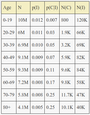
Let’s initially assume a uniform attack rate N(1+)/N(0+) across age – that the true fraction of the population infected does not depend much on age. We can then compare the age distribution of Italy’s confirmed cases to the age distribution of Italy’s population at large to derive an estimate of case under-ascertainment. The idea is that as infection severity increases with age and detection probability increases with severity, the fraction of actual cases detected will increase with age and peak in the elderly. This is a good fit for the data from Italy, where the distribution of observed covid-19 cases is extremely age skewed.

The number of confirmed cases is roughly the probability of testing given infection times the probability of infection times the population size (the net effect of false positive/negative test probabilities are small enough to ignore here):

N(C) = p(C|I)*p(I)*N

From the Diamond Princess data we know that even for the elderly population the fraction of infected who are asymptomatic or mild is probably higher than 50%, so we can estimate that p(C|I) is at most 0.5 for any age group (and would only be that high if everyone with symptoms was tested). Substituting that into the equation above for the eldest 80+ group results in an estimate for p(I) of 0.005 and the following solutions for the rest of the p(C|I) values by age:

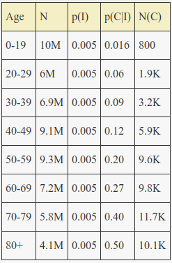
This suggests that the actual total number infected in Italy was at least 0.5% of the population or around ~300,000 true cases as of a week ago or so assuming an average latency between infection and lab confirmation of one week.

Almost all of Italy’s 5K deaths are in the 70-79 and 80+ age brackets, for a confirmed case mortality in those ages of roughly 25%.  This is about 10x higher than observed on the Diamond Princess. Thus a more reasonable estimate for the peak value of p(C|I) is 0.25. Even for the elderly, roughly half of cases are asymptomatic/mild, and half of the remaining are only moderate and do not seek medical care and are not tested. We can also apply a non-uniform attack rate that decreases with age, due to the effects of school transmission and decreasing general infection prone social activity with age.

With an attack rate varying by about 2.5x across age and a max p(C|I) of 0.25, Italy’s total actual infection count is ~566,000 as of a week or so ago – or almost 1% of the population. This is still assuming about double the age 70+ mortality rates observed on the Diamond Princess, so the actual number of cases could be over a million.

Another serious potential confounder is overcounting deaths at the coroner (which I found from this rather good post from the Center for Evidence Based Medicine. Incidentally, the author also reaches my same conclusion about covid-19 IFR ~ influenza IFR):

In the article, Professor Walter Ricciardi,  Scientific Adviser to, Italy’s Minister of Health, reports,  “On re-evaluation by the National Institute of Health, only 12 per cent of death certificates have shown a direct causality from coronavirus, while 88 per cent of patients who have died have at least one pre-morbidity – many had two or three.”

So some difficult-to-estimate chunk of Italy’s death count could be death with covid-19 rather than death from covid-19 (and this also could explain why the average age of covid-19 deaths in Italy is so close to life expectancy).

United States Age Projection

Applying the same last model parameters to the United States general age structure and confirmed covid-19 case age structure results in the following:

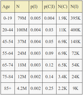
The estimated total number of infections in the US as of a week or so ago is thus ~ 1.1 million, with an estimated overall mortality in the range of 0.1%, similar to the flu. The average mortality in Italy probably is higher partly just because of their age skew. The US has a much larger fraction of population under age 60 with very low mortality.

Assuming that at most 1 in 4 true infections are detected in the elderly, we see that only about 1 in 30 infections are detected in those ages 20-44 and only a tiny fraction of actual infections are detected in children and teens.

Remember the only key assumptions made in this model are:

1. That the attack rate decreases linearly with age by a factor of about 2x from youngest to oldest cohorts, similar to other respiratory viruses (due to behavioral risk differences)
2. That the maximum value of p(C|I) in any age cohort – the maximum fraction of actual infections that are tested and counted, is 0.25.

The first assumption only makes a difference of roughly 2x or so compared to a flat attack rate.

In summary – the age structure of lab confirmed covid-19 cases (the only cases we observe) is highly skewed towards older ages when compared to the population age structure in Italy and the US.  This is most likely due to a sampling selection bias towards detecting severe cases and missing mild and asymptomatic cases – very similar to the well understood selection bias issues for influenza. We can correct for this bias and estimate that the true infection count is roughly 20x higher than confirmed infection count in the US, and about 10x higher than confirmed infection count in Italy.

The Worst Case

In the worst case, the US infection count could scale up by about a factor of 200x from where it was a week or so ago.  With the same age dependent attack rate that would entail everyone under age 20 in the US becoming infected along with 40% of those age 75 and over. Assuming the mortality rates remains the same, the death count would also scale up by a factor of 200x, perhaps approaching 200K. This is about 4x the estimated death toll of the seasonal flu in the US. Yes there is risk the mortality rates could increase if hospitals run out of respirators, but under duress the US can be quite good at solving those types of rapid manufacturing and logistics problems.

However the pessimistic scenario of very high infection rates seems quite unlikely, given:

1. The infection rate of only ~20% on the cramped environment of the Diamond Princess cruise ship
2. The current unprecedented experiment in isolation, sterilization, and quarantine.

A potential critique of the model in the previous section is that we don’t know the true attack rate and it may be different from other known respiratory viruses.  However, this doesn’t actually matter in terms of total death count. We can factor out p(I) as p(I|E)p(E) – the probability of infection is the probability of infection given exposure times the probability of exposure.  A biological mechanism which causes p(I|E) to be very low for the young (to explain their low observed case probability) would result in lower total infection counts and thus higher mortality rates, but it wouldn’t change the maximum total death count – as that is computed by simply scaling up maximum p(E) to 1. So you could replace I with E in the previous model and nothing would change. In other words, that same biological mechanism resulting in lower p(I|E) would also just reduce total infections by the same ratio it increased infected mortality rate, without affecting total deaths.

The Bad News: Current confirmed case count totals (~43K as of today) are a window into the past, as there is about 5 days of incubation period and then at least a few days delay for testing for those lucky enough to get a test. So if the actual infection count was around 1 million a week ago, there could already be more than 5 million infected today, assuming the 30% daily growth trend has continued. So the quarantine was probably too late.

True Costs

Combining estimates for total death count, years of counterfactual life expectancy lost, and about $100k/year for the value of a year of human life from economists we can estimate the total economic damage.

A couple examples using a range of parameter estimates:

• 50k   deaths * 1yr  life lost  * $100k/yr = $5 billion
• 200k deaths * 3yr  life lost  * $100k/yr =  $60 billion
• 500k deaths * 10yr life lost * $100k/yr = $500 billion

In terms of economic damage, the current stock market collapse has erased about 30% of the previous value of ~$80 trillion, for perhaps $23 trillion in economic ‘damage’. I put damage in quotes because trade values can change quickly with expectations, and there is no actual loss in output or capability as of yet. In terms of GDP, some economists give estimates in the range of a 10% to 20% contraction, or $2 to $4 trillion of direct output loss for the US alone.

Although imprecise, these estimates suggest that our current mass quarantine response is expected to do one to two orders of magnitude more economic utility damage than even worst case direct viral deaths.

One silver lining is that much of this economic damage lies in the future predicted.  It can still be avoided when/if it becomes more clear that the death toll will be much lower than original worst case forecasts suggested.

Learning in the Cloud Decentralized

We live in curious times.  Deep Learning is “eating software”, or at the very least becoming the latest trend, the buzziest word.  Its popularity now permeates even into popular culture.

At the same time, GPUs (which power Deep Learning) are in scarce supply due to the fourth great cryptocurrency price bubble/boom (and more specifically due to ether).

All the worlds compute, wasted?

How much computation is all this crypto-mining using?  Most all of it.  As of today the ethereum network is producing around 250 terrahashes/second.  A single GTX 1070 produces around 27 megahashes/second, so currently right this moment there are the equivalent of about 10 million GTX 1070 GPUs dedicated to just ether mining.  This is a 5 terraflop card, so we are talking about around 50 exaflops.  If you include the other cryptocurrencies and roundup, the world is currently utilizing burning roughly a hundred exaflops of general purpose compute for random hashing.  For perspective, the most powerful current supercomputer rates at 1000x less, around 100 petaflops.  So the ether network uses a great deal of compute.  As we will see this in fact is also most of the world’s compute.  The price/cost of this compute is about 3 cents per hour per GTX 1070, or about 600 petaflops/$, or about 8 gigaflops/s/$ amortized over two years.

Buying this much compute up front would cost about ~$10 billion, so we can be reasonable confident that Google or other private companies don’t have compute on this scale.  Firstly, most of the corporate compute capacity is still CPU-based, which has one to two orders of magnitude less flop/$ efficiency and is thus irrelevant.  Secondly, we can more directly estimate GPU corporate compute by just looking at Nvidia’s earnings reports.  It is the main provider, it rather forcefully separates its consumer and corporate product lines, overcharges for the corporate compute by 5x to 10x, and the consumer division still provides most of the revenue.

Google has TPU’s, but they are more specialized for accelerating only dense tensor ops, whereas GPUs are now general accelerators for more arbitrary parallel C++ code.  Each 4 chip TPUv2 accelerator board provides about 180 tflops/s for dense matrix mult for about $7/hour, and thus about 92 petaflops/$, or about 1.3 gigaflops/s/$ amortized over two years.  So google would need to be overcharging by an order of magnitude more than Nvidia is overcharging (very unlikely for various reasons) for the TPUv2 ASIC to be more price effective than a general purpose GPU.  It’s highly unlikely that google has produced anything close to the $10-100 billion worth of TPUv2 hardware required to rival the ether GPU network.  The same analysis applies for microsoft’s limited use of FPGAs, and so on.  Consumer GPUs utterly dominate ops/$, ASICs aren’t yet close to changing that, and Nvidia is already starting to put a TPU-like ASIC on its GPUs anyway with Volta.

Progress in AI ~= Compute spent on AI

“Deep learning requires lots of compute”, although surface level accurate as a statement, doesn’t quite grasp the actual reality.  Many tech business uses of compute have a ‘good enough level’.  There is a certain amount of compute you need to control an elevator, decode a reasonable video stream, parse a web-page, and so on.  Having dramatically more compute than that required is a resource in need of a use.  Many non-technical folks seem to think of compute in these terms.  A perhaps deeper statement would be that Deep Learning is compute.  It is computation directed towards a goal, evolving a system towards some target.  Learning is a computational process.  So there is no ‘good enough’ here, the amount desired is always more.  We can debate what intelligence is a bit, but general intelligence – you know what I mean human – requires continual learning.  In fact, that is perhaps its most defining characteristic.  So intelligence also is (a form of) compute.

If learning is compute, then progress in AI should track growth in compute, which is in fact the case (we could debate what our measure of ‘progress’ is, but let’s not).  The typical ‘start date’ for the deep learning revolution is the first deep CNNs (Alexnet) trained on the large Imagenet database, which also naturally was when someone actually bothered writing and debugging all the code needed to train neural networks in cuda to run on a GPU for the first time.  It was a sudden leap only because there was an effective gap in compute applied to AI/ML due to the end of dennard (clockspeed) scaling and the overhead/delay in moving towards highly parallel programming (aka GPU programming).  Once everyone migrated to GPUs the gap closed and progress continued.

But why has nobody done this yet

Moving to GPUs provided roughly a 10x to 100x one-time boost in compute/$ for AI/ML progress.  There is room for perhaps another 10x or more efficiency jump from algorithm/software level improvements at the tensor math level, but that is another story.  There is a ~5x ish gap between the price of GPU compute on the ether mining network and the low end price of AWS/google/etc cloud compute.  So in theory that gap is large enough for a decentralized AWS like service to significantly outcompete the corporate cloud, take us another large step on the path to AI, and also make a bunch of money.

However, a decentralized compute cloud has some obvious disadvantages:

• Privacy becomes . . . hard
• Requires low-overhead decentralized trust/reliability
• Overall less network bandwidth and higher latency per unit compute
• Potentially more headache to interface

First, let us just ignore privacy for the moment.  There is of course interesting research on that issue, but much of the training use case workload probably doesn’t really require any strong privacy guarantees.  Justifying that statement would entail too many words at the moment, so I’ll leave it for later.  I’ll also assume that the interface issue isn’t really a big deal – like it should be possible to create something on par with the AWS/GCE front end interface for renting a real or virtual machine without much end user hassle but decentralized under the hood.

The reduced network connectivity between node is fundamental, but it also isn’t a showstopper.  Most of the main techniques for parallelizing DL today are large batch data parallel methods which require exchanging/reducing the model parameters at frequency near once per update.  However recent research can achieve up to 500x compression for the distributed communication at the same accuracy, which corresponds to a compute/bandwidth ratio of ~ 22 million flops/ network byte, or about 250 kilobytes/second per 5 terraflop GTX 1070 GPU.  So with SOTA gradient compression, it does look feasible to use standard large batch data parallel training methods across consumer internets.  Even a 100 GPU farm would ‘only’ require gigabit fiber, which is now becoming a thing.  Of course there are other techniques that can reduce bandwidth even farther.  Large-batch data parallelism probably makes the most sense over local ethernet for a GPU farm, but the diminishing returns with larger batch size means at some point you want to evaluate different model variants using something like population level training, or other ‘evolutionary stuff’.  In general given some huge amount of parallel compute (huge relative to the compute required to run one model instance) , you want to both explore numerous model parameter variations in parallel and train the most promising candidates in parallel.  The former form of parallelization uses only small/tiny amounts of bandwidth, and the latter still uses reasonable amounts of bandwidth.  So consumer internet bandwidth limitations are probably not a fundamental issue (ignoring for the moment the engineering challenges).

So that leaves us with the issue of trust or reliability.  If you rent a TPU/GPU on GCE/AWS, you can reasonably trust that 1.) it will compute what you want it to, and 2.) it won’t leak your precious code/model/data whatever to unscrupulous rivals/ISIS etc.  Again at the moment lets leave out issue 2.) and focus on reliable computation.

The ideal crypto approach to solving reliability involves trustless automated (dumb) mechanisms: ideally an algorithm running on the blockchain something something with some nice proofs that workers can’t find exploits to get paid for fake/forged work or at least that any such exploit is unprofitable.  Truebit is probably a good example of SOTA for this approach.  Truebit’s full solution is rather complex, but basically task providers submit tasks on the blockchain, workers claim solutions, and verifiers and judges arbitrate disputes using log(N) binary search between merkle trees of workers and verifiers.  The scheme induces extra compute overhead for recomputing tasks redundantly across workers and verifiers and also considerable network/blockchain bookkeeping overhead.  The authors estimate that the overhead for all this is on the order of 500% to 5000%  (section 4.2).  Unfortunately this is far too much.  The decentralized cloud has hope for a a 5x compute/cost efficiency advantage in the zero overhead case, and it has some inherent disadvantages (cough privacy).  So really the overhead needs to be less than 200% to be competitive, and ideally much less than that.  If anyone is actually planning a business case around a truebit based solution actually competing with the corporate cloud in general, they are in for a rude awakening.  End users of bulk compute will not use your system just because it is crypto/decentralized, that is not actually an advantage.

In the following technical part of this post I’ll describe some partially baked ideas for improving over Truebit and moving closer to the grail of epsilon overhead even in the ideal ‘trustless’ crypto model.  However, before getting in to that, I should point out that the common sense solution to this problem may actually be the best, business wise.  By common sense here I mean “whatever actually works”, rather than what works subject to some imagined constraints such as in the trustless crypto model.  As far as I know, Amazon does not offer a reliability proof for the compute it sells on AWS, but it still works just fine as a business.  So the simplest low overhead (ie actually usable) solutions to trust for decentralized computing probably look more like AirBnB than proof-of-work.  Instead of trying to get machines to automate something hard that humans can do reasonably easily . . . just have humans do it.

To unpack that idea, consider the conditions leading to clients trusting AWS.  As far as I know, AWS has not yet attempted computational fraud on any large scale.  Yet it would be easy for them to do so .. they could sell 10% of a machine’s compute resources and claim the user is getting 50%, for example.  What prevents this?  Competition and reputation.  Competition is easy to achieve in a crypto-system, hard to avoid actually.  Reputation, on the other hand, is a bit trickier.  One of the key ideas in crypto land is that everyone is anonymous and nodes can join/depart at will – which obviously prevents any significant build up of or reliance on reputation.  But there is no fundemental reason for this in the context of a cloud computing grid.  Do the (human) compute providers really need to be anonymous?  Probably not.  So a reputation solution is probably the most net efficient here.  AirBnB or Ebay work just fine running reputation and arbitration computations mostly on human minds.  Of course, reputation is also something perhaps that increasingly can be automated to various degrees (ie, uport).  Golem is also apparently relying on a partially automated reputation system.

So after acknowledging that fully general automatic trustless secure outsourced computation may be impossibly hard; and perhaps unnecessary given workable ‘hacky’ alternatives, let’s give it a shot anyway.

The Verification Problem

A core problem in outsourced computation is verification:  automatically determining whether the claimed output of a function is actually correct.  If we involve multiple parties (which seems necessary) this just becomes another form of generalized consensus.  The setup: we have a number of agents which can communicate facts in some formal logic like language; agents have limited knowledge; agents can lie (make statements for which they can locally prove to be false) , and we seek efficient algorithms agents can use to determine the truthhood of a statement, or at least estimate the probability thereof, subject to some convergence constraint.  Naturally this is a big complex problem.  A key component of any solution usually (necessarily?) involves a verification game played by two or more agents.  The game is a contest over the veracity of a statement, the outcome of the game provides key evidence agents can use to update their beliefs (assuming the agents are bayesian/probabilistic, in the weaker model where agents are dumb non-probabilistic reasoners, updates are of course binary).

Consider the specific example where Alice hires Bob to render an image using some expensive ray tracing function.  We can describe this as:

Alice -> { if (Bob->{ this, #Y } : Y = F(X)) then Alice -> { send(coin3423, Bob) } }

In other words, Alice says that if Bob says (provides) Y, such that Y = F(X), then Alice sends a coin to Bob.  This is a contract that Alice signs and sends to Bob who can then compute Y and sign the hash of Y appended to the contract (this) to make a payment claim.  Bob can then provide this contract claim to any third party to prove that Bob now owns coin3423.  You get the idea.

Suppose in this example that X is an input image (identified by a hash of course), F describes the fancy ray tracing function, and Y is the output image.  To redeem the coin Bob ‘earned’, Bob needs to send the signed contract thing to some other party, Charlie.  This new party then faces a verification burden: Bob is the legitimate owner of the coin iff #Y is a valid hash of the output of F(X), which requires that Charlie recompute F(X).  Assume we already have some mechanism to prove ownership of the coin previous to this new statement, then the verification burden is still quite high: F(X) needs to be recomputed on order O(T) times, where T is the subsequent number of transactions, or alternatively F(X) needs to be recomputed O(N) times, where N is the number of peers in a consensus round.  This is basically how verification works in systems like ethereum and why they don’t really scale.

We can do much better in some cases by breaking the function apart.  For example, in the ray tracing example, F(X) is highly parallel: it can be decomposed like so F(X) = Y[i] = F(X[i]), where i is an index over the image location.  The global function decomposes simply into a single large parallel loop over independent functions: it is trivially parallelizable.

In this scenario a probabilistic verification game can converge to e accuracy in just one iteration using order -log(e) subcomputations/subqueries, which is a huge improvement: or more specifically the burden is only ~ -log(e) / N, where N is the parallel width and e is an error (false positive) probability.  For example, instead of recomputing all of F(X), Alice or Charlie can just pick a handful or i values randomly, and only recompute F(X[i]) at those indices.  If Bob faked the entire computation, then verifying any single index/pixel sub-computation will suffice.  If Bob faked 60%, then testing k locations will result in a (1.0 – 0.6)^k probability of false positive, and so on.  So the parallel parts of a computation graph permit efficient/scalable probabilistic verification games.  But this doesn’t work for serial computation.  What we need is some way to ‘unchain’ the verification, hence the name of this idea.

Unchained Deterministic Trustless Verification

Consider a serial function of the form Y[i+1] = F(Y[i]).   Assume we have access to a fast probabilistic micropayment scheme.  Instead of one contract conditional on the overall function, Alice decomposes that into a larger number of probabilistic micropyaments conditional on each sub-computation in the graph, at some granularity.  The probabilistic micropayment can just be a payment conditional on a timelocked random process (something nobody could know now, but becomes easy to know in the future, such as the hash of some future ether block).  Now the wierd part: instead of contracting on the ‘correct’ inputs to every subcomputation (which Alice doesn’t know without computing the function in the first place), Alice allows Bob to pick them.  For every subcomputation, Bob claims what the inputs and output were at that step, wraps that up in a hash commitment, and exchanges that for a tiny p-payment with Alice.  At the time of the exchange neither Alice nor Bob knows which of the p-payments (lottery tickets) will actually cash out in the future.  Bob keeps the p-payments and checks them in the future.  Some tiny fraction of them are winners, and Bob then ‘claims’ just those coins by using them in a transaction (sending them to Charlie say), which then requires verification – but crucially – it only requires verification of that one sub-computation, independent of the whole graph.  Thus the chain has been broken.  The cost of verification can be made rather arbitrarily small up to the limits of the p-payment scheme, because now only a fraction of the computations matter and require subsequent verification.

Unfortunately this doesn’t quite work as stated, at least not for all functions.  Instead of computing the function on the actual inputs, Bob could instead substitute some other inputs.  For example, instead of computing and signing Y[i+1] = F(Y[i]), Bob could compute and claim Y[i+1] = F(trash).  This is valid because the unchaing necessarily broke the dependencies which constrain the inputs – Bob can pick the inputs.  In a typical scenario the sub-computations will repeat heavily, so Bob could get a big savings by computing each newly encountered sub-function once, memorizing the inputs, and then recycling those over and over.  Let us call this the memoization attack.

Fortunately there is a modification which seems to make it all work again, at least for certain functions.  In machine learning all operations which cost anything are tensor operations on large arrays of real values.  In this setting, Alice can submit a special small seed input for a noise function which Bob is required to add to each input.  So each contract job now is something like Y[i+1] = F(Y[i] + noise(a[i])), where noise is some known good fast deterministic noise generator, and a[i] is a seed alice picks.  Note that the seeds can be chained and even the whole decomposition into subtransactions can be implicitly compressed to save any bandwidth cost.

The noise should be small enough such that it doesn’t hurt the overall learning process (which is easy enough, some amount of noise injection is actually useful/required in DL), but still just large enough to always effect the output hash.  The noise inputs from Alice prevents Bob from using memoization and related attacks.  In fact, if the function F is ‘hard’ in the sense that the fastest algorithm to compute F for input X + noise takes the same running time for all X, then Bob has nothing to gain by cheating.  On the other hand, if there are algorithms for F which are must faster for particular inputs then the situation is more complex.  For example, consider matrix multiplication.  If we constrain the outputs to fairly high precision (say at least 32 bit FP say), then it seems likely that only a small noise pertubation is required to force Bob to use dense matrix multiplication (which has the same run time for all inputs).  However as we lower the required output precision, then the noise variance must increase for dense matrix multiplication to still be the fastest option.  For example if the hash only requires say 8 bits of output precision and the noise is very small, Bob may be able to compute the output faster by quantizing the input matrices and using a sparse matrix multiply which may take much less time on zero + noise than X + noise (X being the correct input).  The noise must be large enough such that it changes some reasonable number of output bits for even the worst fake inputs Bob could pick (such as all zeroes).

Now in practice today dense matrix multiplication with 16 or 32 bit floating point is dominant in machine learning; but dense matrix mult is solved and the harder sparse case continues to improve, so naturally a scheme that only works for dumb/hashlike subfunctions is not ideal.  However, for an early half-baked idea I suspect this line of attack has some merit and perhaps could be improved/extended to better handle compression/sparsity etc.

 

All payments are bets

Another interesting direction is to replace the basic “p-payment conditioned on correct output” style contract with a bidirectional bet on the output.  Alice sends Bob requests which could be in the form of “here is a function I would be on: F(X)”, and Bob sends back a more concrete “I bet 100 coins to your 1 that F(X)=Y”.  Having Bob put up funds to risk (a kind of deposit) strengthens everything.  Furthemore, we could just extend bets all the way down as the core verification/consensus system itself.

Good Bob computes Y=F(X), Bad Bob computes Y != F(X) but claims Y=F(X).  Bob then tries to claim a resulting coin – spend it with Charlie.  Charlie needs to evaluate the claim Y = F(X) … or does she?  Suppose instead that Charlie is a probabilistic reasoner.  Charlie could then just assign a probability to the statement, compute expected values, and use value of information to guide any verification games.  You don’t avoid verification queries, but probabilistic reasoning can probably reduce them dramatically.  Instead of recomputing the function F(X), Charlie could instead use some simpler faster predictive model to estimate p(Y = F(X)).  In the case where the p value here is certainly large enough, then further verification is financially/computationally unjustified.  Charlie can just discount the expected value of the coin slightly to account for the probability of fraud.  Charlie can pass the coin on with or without further verification, depending on how the expected values work out.  Better yet, instead of doing any of the actual expensive verification, Charlie could solicit bets from knowledgeable peers.  Verification is then mostly solved by a market over the space of computable facts of interest in the system.  Investigation – occasionally verifying stuff in detail by redoing computations – becomes a rare occurrence outsourced to specialists.  I suspect that the full general solution to consensus ends up requiring something like this.

This is more like how the real world works.  Purchasing a property does not entail verifying the entire chain of ownership.  Verification always bottoms at some point where the cost is no longer justified.  Naturally this leads to a situation where fraud is sometimes profitable or at least goes undetected, but it is far from obvious that this is actually undesirable.  One possible concern is Black Swans: some large fraud that goes undetected for a long time only to be revealed later causing a complex unwinding of contracts and payments.  A natural solution to this is to bottom out complex contractual chains by swaps or conditional overwrites.  For example, any of the conditional payment mechanisms discussed earlier should have a third option wherein if both parties agree/sign to a particular outcome than that short-circuits the bet condition and thus prevents graph complexity explosion.  To this we can append a dispute resolution chain using a hierarchy of increasingly slower/larger/more trustworthy entities, using predesignated arbiters and so on, such that all ownership chains simplify over time.  This also happens to be a solution feature we see in the real world (arbitration/judicial review hierarchies).

Arbiter Networks: Simple Low-Latency Scalable Micropayments sans Channels

Current blockchain networks (Bitcoin, Ethereum, etc.) do not scale efficiently: their per transaction cost is ~O(N), where N is the number of full nodes.  Several recent proposals provide restricted fast O(C) transactions using combinations of payment channels, probabilistic payments, and either cross channel routing (Lightning Network), or surety bonds/deposits to deter double-spending.  I propose a new delegated arbitration mechanism wherein payees predetermine third party arbiters who quickly resolve double-spending disputes instead of predetermining the payee as in payment channels.  Arbiters can prove honesty through penal bond precommitments and compete to earn small transaction fees in exchange for their services.  Delegated arbitration eliminates the need for most users to lock up money in numerous channel deposits or bonds, more effectively allocates the net savings of the network, and in combination with unbound probabilistic payments allows for a high throughput and minimal latency micropayment network.

Note: I wrote up an earlier version of this in 2014, but didn’t finally get around to publishing it here until now.  This blog post is a informal precursor to a research paper and will be light on details.

Background

Blockchain scalability was a primarily a theoretical problem that was mostly ignored by the non-technical community up until recently.  Bitcoin and all other blockchain based cryptocurrency networks are simple full replica systems: each transaction is processed redundantly by all full network nodes.  Thus the per transaction cost is O(N), which does not scale efficiently (the bandwidth cost per transaction increases as the network grows).    However, in theory blockchain networks can effectively be O(C) if almost all network agents run “light clients” and the number of full nodes is constrained to a reasonable constant.  In practice, this still works out to a prohibitively large O(C) constant.

Payment channels are a simple technique that can solve double-spending for the restricted payment stream setting.  If Alice anticipates sending some large unknown number of small micropayments to Bob in the future, Alice can lock up some money into a channel that either pays only to Bob or refunds back to Alice after some reasonable timeout.  Double spending is prevented because … the channel locks the payee field to a set of size one.  The disadvantage is Alice must anticipate future spending and lock up sufficient funds.  The timeout mechanism can also be complex.

Probabilistic payments are a micropayment mechanism investigated for decades preceding the arrival of Bitcoin. Each probabilistic payment uses a lottery ticket which has the same expected value as a larger regular macropayment, but that value is concentrated in a few rare tickets.  Most tickets have zero value and are discarded, greatly reducing transaction tracking overhead.  Probabilistic payments require a secure multi-party RNG.  If a public RNG is available (such as hashes of the future bitcoin blockchain state itself), then generic lottery tickets can be used which pay to any holder and don’t require locking up funds in a channel with a particular payee.  These more generic lottery tickets are essentially prediction market shares where the bet is on an RNG value.  Conceptually the setup transaction is something like “if (rng % K == B), pay to Alice.Temp[B], else pay to Alice”.  Then to pay Bob a lottery ticket, Alice just sends Alice.Temp[B] to Bob.  The setup transaction divides a deterministic coin into K unique probabilistic coins (lottery tickets).

Probabilistic payments can alternatively involve a local RNG where the payer and payee use a two-party crytpo random number protocol to setup a lottery ticket.  However there is no way in general to overcome the fundamental limitations of multi-party computation: one party can always gain some edge by defecting from any step in the exchange of secrets.  There are various complex ways to mitigate this like splitting the secrets up into many small bits, or using a third party, but at that point you might as well just rely on the third party RNG variant in the first place.  On the other hand, in a micropayment setting where parties are conducting large numbers of consecutive small transactions game theory works in our favour and small defections may not matter.

Note that probabilistic payments alone do not solve double spending; the generic multi-party variant can easily be double-spent, and the two party channel variant can prevent double-spending only through the channel lock mechanism.  But if you are already using payments channels, you could just consolidate stream transactions (a sequence of A->B transactions for different amounts later get replaced with a single larger transaction).  This provides the same benefits as channel bound probabilistic payments with perhaps less complexity.

The Lightning Network is an offchain micropayment protocol that adds a routing network layer on top of payment channels.  Each payment channel forms a node in a network.  Arbitrary payments between any two agents can then be routed across this network in a vaguely onion routing like fashion.  Channel transactions are O(C), which is great, but all channel setup transactions, dispute transactions, timeouts, etc all still require full transactions (on-chain) which are still O(N) when using a blockchain network as the underlying foundation.  So the lightning network is not really O(C) in expectation unless the average ratio of on-channel (off-chain) transactions to full (on-chain) transactions is O(N), which seems dubious.  Furthermore, multi-hop routing in the lightning network adds latency similar to onion routing in TOR, which is potentially a significant disadvantage for latency-sensitive applications.  The lightning network also requires all parties to lock up funds in channels for micropayments, essentially tying the economic network and the physical communication network together.

Penal bonds (aka security deposits) are a simple game-theoretic mechanism that allow honest agents to credibly signal their honesty by precomitting to an economic penalty for dishonest behaviour.  Bonds themselves are a proposed potential solution for double-spending, and more recently Chiesa et all propose using a combination of bonds(deposits) and probabilistic payments in “Decentralized Anonymous Micropayments” (DAM).

To guarantee a negative payout for any double-spending attack the bond/deposit must be larger than the integral of the network’s entire GDP over the length of time required to detect double spending.  In the worst case the payout for an optimal double spend is bound by the maximum value the network can ‘produce’ in the time window of detection  (in other words, the optimal double-spending attack generates effectively infinite but very temporary wealth that can only purchase the very finite amount of services or stuff the network offers for the time period).  For the case of a hypothetical network that produces $1 billion a year of various compute services and a 10 minute double-spend detection window, the safe bond/deposit size is on order $20,000 – fairly prohibitive.  A double-spend detection window of just 3 seconds still works out to a $100 bond/deposit value.  The situation worsens considerably when we consider external exchanges and short-timescale fluctuations.

Unfortunately “detecting double-spends” is itself not something that can easily be done in O(C) per transaction.  So any bond/deposit solution that still requires payees to monitor all micropayments on the underlying blockchain network obviously can not actually be a solution itself.  However, combinations of bonds (to deter double spending) and probabilistic payments (to reduce the overhead of detecting double-spending) are a viable micropayment solution.  DAM uses bound two-party probabilistic payments + bonds + stuff (for anonymity), Arbiter Networks uses unbound probabilistic payments + bonds + delegated arbitration.  Making arbiter networks natively anonymous is beyond the scope of this post, and perhaps unimportant given future improvements to off-chain mixing protocols.

Method Overview

Arbiter networks provide O(C) scalable micropayments sans channels through delegated arbitration: the task of resolving double-spending disputes is delegated to third party arbiters who otherwise have no actual transaction authority (no multi-sig and thus no counterparty risk if the arbiter fails).  Arbiters use sufficiently sized penal bonds to provably signal honesty and can charge small transaction fees for their services.  Essentially arbiters rent out the economic utility of their bond, allowing more agents to participate without investing in bonds (as compared to pure bond/deposit schemes).  In essence, delegated arbitration is an add-on improvement to any bond/deposit mechanism.

A payer first sends money into a special account/contract that specifies a third party arbiter who resolves any equivocation/fraud (ie double-spending) disputes for those funds, but does not lock up the payee (unlike channels).  Subsequent transactions involve only the payer, any arbitrary payee, and the predetermined arbiter.  The payer sends payment information directly to the payee and arbiter, the arbiter checks for double-spend/fraud/errors then forwards the payment confirmation information to the payee.  Upon receiving confirmation from the arbiter the payee can trust that the payer has not double spent so long as the arbiter’s penal bond is valid and of sufficient size to provably deter any double-spending from a hypothetical payee/arbiter collusion.

A timeout mechanism allows return of funds for the case of a non-responsive arbiter, as in payment channel timeout in Lightning Network.  Payment channels lock the payee field, but delegated arbitration only locks the arbiter of disputes without locking the payee.  Thus all the headaches of locking up funds into various channels in Lightning is avoided, and more importantly, transactions are routed through a near minimal 2 hop path for low latency and high throughput.

Arbiter Networks and Lightning Network both provide a constant speedup in transaction throughput and reduction in transaction cost.  The Arbiter Network speedup is determined by the average factor (K/2): the number of probabilistic micropayments per macropayment (which is ultimately bound only by payee volatility tolerance).  Only macropayments hit the full underlying network.  The constant speedup for Lightning Network is some other factor (R/T): where R is the ratio of micropayments across a channel to macropayments to setup or refund a channel and T is the average number of hops in a route.  I expect that (K/2) > (R/T), and moreover that K > R, but showing this will require some rather detailed thought experiments or simulations to substantiate.

Multi-Party Secure RNG

Any underlying blockchain can be used as an approximately ideal secure RNG.  The hash value of  some future block (T+C) are essentially unknowable to any party at block time T under realistic conditions.  The situations where this condition fails are those where one party effectively has far more hash power than the rest of the network combined, and can afford to sit on a long extended chain for a time period of C.

A disadvantage of using a blockchain as the RNG is naturally that it does require monitoring the underlying blockchain network, but even this cost could be mitigated by having “blockchain summarizers” who monitor the blockchain network and publish the vastly smaller hashes of blocks in exchange for some small fee.  These summarizers could naturally be kept honest through penal bonds, as the work they perform is easily verifiable.

Consider an example worker agent that sells one high end GPU worth of compute services.  This agent could expect to earn perhaps $5 per day.  Current transaction fees in both bitcoin and ethereum average around $1 (which does not include the miner subsidy).  Thus a realistic value of K (the number of lottery tickets per coin, or micro to macro) should be balanced to have at most one macropayment per day on average.  For an average rate of about 10 microtransactions per second (which seems reasonable for many applications), this works out to a K value of roughly 1 million.  In practice a typical worker agent will probably have more than one GPU, although a fee overhead of 20% is also perhaps unrealistically high.

Market Arbitration Rates

There is an interesting connection between interest rates and the fees which arbiters can expect to charge.  An arbiter is essentially renting out the utility of their penal bond.  This locks up money that could otherwise be spent or invested in some computation, or could be lent out at interest.  Curiously, the presence of penal bonds itself creates a need or niche for loans: bond holders may find themselves short of free cash but they have the bond as collateral.  Loan repayment could be contractually automated such that the only risk a lendee undertakes when loaning to a bond-holder is the risk of bond default in the interim due to malfeasance.  Normally this risk should be very low for adequately sized bonds, so the loan rate for these secured loans should be close to the risk free interest rate.  So now there are actually at least two options for coin holders to earn low risk return: they can lock up coins in a bond and earn transaction fees or rent out their coins.  (Financial markets provide another market for coin loans for instruments such as short contracts).

As the various uses of cash compete, the rate of return should normalize between the various uses.  Thus the rate of return on a bond should be similar to some sort of natural low-risk interest rate.  Transaction fees could be estimated from this if one knew the typical velocity of money: ie R = r^V, where R is the rate of return per year or time period, r is the average rate of return per transaction, and V is the transaction rate (per time period).  For example, if we assume R is 1% per year (reasonable), and V is 32 transactions per second or about 1 billion transactions per year, then r is about 10^-9.  For a bond of size $1,000 (reasonable from earlier analysis), this works out to fixed transaction fees of about 1 millionth of a dollar.  In simpler terms, agents who lack bonds should expect to pay transaction fees on order of the interest rate for renting the bond for the equivalent time period of their transaction volume.  In this fictional example the arbitration fees are on order similar to the macropayment transaction fees, which seems vaguely reasonable.

As the arbitration fees depend on the bond sizes which depend crucially on the double spend detection window time, a faster double-spend detection mechanism could be important (faster than just checking the macro-payments on the blockchain).  I leave that to a future work.

Conclusion

The world altering decentralized applications of the future all involve a computational economy: a sea of autonomous machines bidding, contracting, and competing to perform useful computations.  All economies require a currency as their lifeblood; crypto-currency is the natural choice for a future virtual compute economy, but sadly current crypto-currency systems are simply not up to the task.  However, a rather straightforward combination of simple mechanisms can probably get us most of the way there.  This Arbiter Network proposal is a potential piece of a larger vision I hope to explore soon in subsequent posts.

 

Articles from 2015/2016

My most recent writings can be found on LessWrong.  I wrote there rather than here mostly due to the LW/reddit codebase’s superior support for comments and the ready supply of comments/commenters (at least historically – it has been dying).

Perhaps the best article I’ve written in a while is The Brain as a Universal Learning Machine, but The Unfriendly Superintelligence next door isn’t bad either.

Dark Extraterrestrial Intelligence

In regards to the Fermi Paradox there is a belief common in transhumanist circles that the lack of ‘obvious’ galactic colonization is strong evidence that we are alone, civilization is rare, and thus there is some form of Great Filter.  This viewpoint was espoused early on by writers such as Moravec, Kurzweil, and Hanson; it remains dominant today.  It is based on an outdated, physically unrealistic model of the long term future of computational intelligence.

The core question depends on the interplay between two rather complex speculations: the first being our historical model of the galaxy, the second being our predictive model for advanced civilization.  The argument from Kurzweil/Moravec starts with a type of manifest destiny view of postbiological life: that the ultimate goal of advanced civilization is to convert the universe into mind (ie computronium).  The analysis then precedes to predict that properly civilized galaxies will fully utilize available energy via mega-engineering projects such as dyson spheres, and that this transformation could manifest as a wave of colonization which grows outward at near the speed of light via very fast replicating von-neumann probes.

Hundreds of years from now this line of reasoning may seem as quaint to our posthuman descendants as the 19th century notion of martians launching an invasion of earth via interplanetary cannons.  My critique in two parts will focus on: 1.) Manifest Destiny Transhumanism is unreasonablely confident in its rather specific predictions for the shape of postbiological civilization, and 2.) the inference step used to combine the prior historical model (which generates the spatio-temporal prior distribution for advanced civs) with the future predictive model (which generates the expectation distribution) is unsound.

Advanced Civilizations and the Physical Limits of Computation

Imagine an engineering challenge where we are given a huge bag of advanced lego-like building blocks and tasked with organizing them into a computer that maximizes performance on some aggregate of benchmarks.  Our supply of lego pieces is distributed according to some simple random model that is completely unrelated to the task at hand.  Now imagine if we had unlimited time to explore all the various solutions.  It would be extremely unlikely that the optimal solutions would use 100% of available lego resources.  Without going into vastly more specific details, all we can say in general is that lego utilization of optimal solutions will be somewhere between 0 and 1.

Optimizing for ‘intelligence’ does not imply optimizing for ‘matter utilization’.  They are completely different criteria.

Fortunately we do know enough today about the limits of computation according to current physics to make some slightly more informed guesses about the shape of advanced civs.

The key limiting factor is the Landauer Limit, which places a lower bound of (kT ln 2) on any computation which involves the erasure of one bit of information (such as overwriting 1 bit in a register).  The Landauer Principle is well supported both theoretically and experimentally and should be non-controversial.  The practical limit for reliable computing is somewhat larger: in the vicinity of 100kT, and modern chips are already approaching the Landauer Limit which will coincide with the inglorious end of Moore’s Law in roughly a decade or so.

The interesting question is then : what next?  Moving to 3D chips is already underway and will offer some reasonable fixed gains in reducing the Von Neumman bottleneck, wire delay and so on, but it doesn’t in anyway circumvent the fundamental barrier.  The only long term solution (in terms of offering many further order of magnitude increases in performance/watt) is moving to reversible computing.  Quantum computing is the other direction and is closely related in the sense that making large-scale general quantum computation possible appears to require the same careful control over entropy to prevent decoherence and thus also depends on reversible computing.  This is not to say that every quantum computer design is fully reversible, but in practice the two paths are heavily intertwined.

A full discussion of reversible computing and its feasibility is beyond my current scope (google search: “mike frank reversible computing”); instead I will attempt to paint a useful high level abstraction.

The essence of computation is predictable control.  The enemy of control is noise.  A modern solid-state IC is essentially a highly organized crystal that can reliably send electronic signals between micro-components.  As everything shrinks you can fit more components into the same space, but the noise problems increase.  Noise is not uniformly distributed across spatial scales.  In particular there is a sea of noise at the molecular scale in the form of random thermal vibrations.  The Landauer Limit arises from applying statistical mechanics to analyze the thermal noise distribution.  You can do a similar analysis for quantum noise and you get another distinct, but related limit.

Galactic Real Estate and the Zones of Intelligence

Notice that the Landauer Limit scales linearly with temperature, and thus one can get a straightforward gain from simply computing at lower temperatures, but this understates the importance of thermal noise.  We know that reversible computing is theoretically possible and there doesn’t appear to be any upper limit to energy efficiency – as long as we have uses for logically reversible computations (and since physics is reversible it follows that general AI algorithms – as predictors of physics – should exist in reversible forms).

The practical engineering limits of computational efficiency depend on the noise barrier and the extent to which the computer can be isolated from the chaos of its surrounding environment.  Our first glimpses of reversible computing today with electronic signalling appear to all require superconducting, simply because without superconducting wire losses defeat the entire point.  A handful of materials superconduct at room temperature, but for the most part its a low temp phenomenon.  As another example, our current silicon computers work pretty well up to around 100C or so, around which failures become untenable.  Current chips wouldn’t work too well on venus.  Its difficult to imagine an effecient computer that could work on the surface of the sun.

Now following this logic all the way down, we can see that 2.7K (the cosmic background temperature) opens up a vastly wider space of advanced reversible computing designs that are impossible at 270K (earth temperatures), beyond the simple linear 100x efficiency gain.  The most advanced computational intelligences are extraordinarily delicate in direct proportion.  The ideal environment for postbiological super-intelligences is a heavily shielded home utterly devoid of heat(chaos).

Visualizing temperature across the universe as the analog of real estate desirability naturally leads to a Copernican paradigm shift.  Temperature imposes something like a natural IQ barrier field that repulses postbiological civilization.  Life first evolves in the heat bath of stars but then eventually migrates outwards into the interstellar medium, and perhaps eventually into cold molecular clouds or the intergalactic voids.

Bodies in the Oort Cloud have an estimated temperature in the balmy range of around 4-5K, and thus may represent the borderline habitable region for advanced minds.

Dark Matter and Cold Intelligences

Recent developments concerning the dark matter conundrum in cosmology can help shed some light on the amount of dark interstellar mass floating around between stars.  Most of the ‘missing’ dark matter is currently believed to be non-baryonic, but these models still leave open a wide range of possible ratios between bright star-proximate mass and dark interstellar mass.  More recently some astronomers have focused specifically on rogue/nomadic planets directly, with estimates ranging from around 2 rogue planets per visible star[1] up to a ratio of 100,000 rogues to regular planets.[2]  The variance in these numbers suggests we still have much to learn on this question, but unquestionably the trend points towards a favorably large amount of baryonic mass free floating in the interstellar medium.

My current discussion has focused on a class of models for postbiological life that we could describe as cold solid state civilizations.  Its quite possible that even more exotic forms of matter – such as dark matter/energy enable even greater computational efficiency.  At this early stage the composition of non-baryonic dark matter is still an open problem and its difficult to get any sense for the probability that it turns out to be useful for computation.

Cold dark intelligences would still require energy, but increasingly less in proportion to their technological sophistication and noise isolation (coldness).  Artificial fusion or even antimatter batteries could provide local energy, ultimately sourced from solar power harvested closer to the low IQ zone surrounding stars and then shipped out-system.  Energy may not even be a key constraint (in comparison to rare elements, for example).

Cosmological Abiogenesis Models

For all we know our galaxy could already be fully populated with a vast sea of dark civilizations.  Intelligence and technology far beyond ours requires ever sophisticated noise isolation and thermal efficiency which necessarily corresponds to reduced visibility.  Our observations to date are certainly compatible with a well populated galaxy, but they are also compatible with an empty galaxy.  We can now detect interstellar bodies and thus have recently discovered that the spaces between stars are likely teeming with an assortment of brown dwarfs, rogue planets and (perhaps) dark dragons.

In lieu of actually making contact (which could take hundreds of years if they exist but deem us currently uninteresting/unworthy/incommunicable), our next best bet is to form a big detailed bayesian model that hopefully outputs some useful probability distribution.  In a sense that is what our brains do to some approximation, but only with some caveats and gotchas.

In this particular case we have a couple of variables which we can measure directly – namely we know roughly how many stars and thus planetary systems exist: on the order of 10^11 stars in the milky way.  Recent observations combined with simulations suggest a much larger number of planets, mostly now free-floating, but in general we are still talking about many billions of potentially life-hospitable worlds.

Concerning abiogenesis itself, the traditional view holds that life evolved on earth shortly after its formation.  The alternative is that simple life first evolved .. elsewhere (exogenesis/panspermia).  The alternative view has gained ground recently: robustness of life experiments, vanishing time window for abiogenesis on earth, discovery of organic precursor molecules in interstellar clouds, and more recently general arguments from models of evolution.

The following image from “Life Before Earth” succinctly conveys the paper’s essence:

Even if the specific model in this paper is wrong (and it has certainly engendered some criticism) the general idea of fitting genomic complexity to a temporal model and using that to estimate the origin is interesting and (probably) sound.

What all of this suggests is that life could be common, and it is difficult to justify a probability distribution over life in the galaxy that just so happens to cancel out the massive number of habitable worlds.  If life really is about 9 billion-ish years old as suggested by this model it changes our view of life evolving rarely and separately as a distinct process on isolated planets to a model where simple early life evolves and spreads throughout the galaxy with a transition from some common interstellar precursor to planet-specialized species around 4 billion years ago.  There would naturally be some variance in the time course of events and rate of evolution on each planet.  For example if the ‘rate of evolution’ has a variance of 1% across planets – that would correspond to a variance of about 40 million years for the history from prokaryotes to humans.

If we could see the history of the galaxy unfold from an omniscient viewpoint, perhaps we’d find the earliest civilization appeared 100 million years ago (2 standard devs early) and colonized much of the high value real estate long before dinofelis hunted homo habilis on earth.

In light of all this, the presumptions behind the Great Filter and the Fermi ‘Paradox’ become less tenable.  Abiogenesis is probably not the filter.  There still could be a filter around the multicellular transition or linguistic intelligence, but not in all models.  Increasingly it looks like human brains are just scaled up hominid brains – there is nothing that stands out as the ‘secret sauce’ to our supposedly unique intelligence.  In some of the modern ‘system’ models of evolution (of which the above paper is an example) the major developmental events in our history are expected attractors, something like the main sequence of biological evolution.  Those models all output an extremely high probability that the galaxy is already colonized by dark alien superintelligences.

Our observations today don’t completely rule out stellar-transforming alien civs, but they provide pretty reasonable evidence that our galaxy has not been extensively colonized by aliens who like to hang out close to stars and capture most of that energy and or visibly transform the system.  In the first part of the article I explored the ultimate limits of computing and how they suggest that advanced civilizations will be dark and that the prime real estate is everywhere other than near stars.

However we could have reached the same conclusion independently by doing a Bayesian update on the discrepancy between the high prior for abundant life, the traditional Stellar Engineering model of post-biological life, and the observational evidence against that model.  The Bayesian thing to do in this situation is infer (in proportion to the strength of our evidence) that the traditional model of post-biological life is probably wrong, in favor of new models.

So, Where are They?

The net effect of the dark intelligence model and our current observations is that we should update in favor of all compatible answers to the fermi paradox, which namely include the simple “they are everywhere and have already made/attempted contact”, and “they are everywhere and have ignored us”.

As an aside, its interesting to note that some of the more interesting SETI signal candidates (such as SHGb02+14a) appear to emanate from interstellar space rather than a star – which is usually viewed as negative evidence for intelligent origin.

Seriously considering the possibility that aliens have been here all along is not an easy mental challenge.  The UFO phenomenon is mostly noise, but is it all noise?  Hard to say.  In the end it all depends on what our models say the prior for aliens should be and how confident we are in those models vs our currently favored historical narrative.